
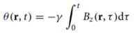
In MRI, we receive a volume integral from an array of oscillators. By ensuring that the phase,“signature” of each oscillator is unique, one can assign a unique location to each spin and thereby reconstruct an image. During signal reception, the applied magnetic field points in the z direction. Spins precess in the xy plane at the Larmor frequency. Hence a spin at position r = (x, y,z) has a unique phase θ that describes its angle relative to the y axis in the xy plane:
where Bz(r, t) is the z component of the instantaneous, local magnetic flux density. This formula assumes there are no x and y field components.
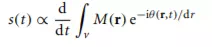
A coil large enough to receive a time-varying flux uniformly from the entire volume produces an EMF proportional to
where M(r) represents the equilibrium moment density at each point r.
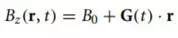
The key idea for imaging is to superimpose a linear field gradient on the static field B0. This field points in the direction z, and its magnitude varies linearly with a coordinate direction. For example, an x gradient points in the z direction and varies along the coordinate x. This is described by the vector field xGx zˆ, where ž is the unit vector in the z direction. In general, the gradient is (xGx + yGy + zGz)ž, which can be written compactly as the dot product G · rž. These gradient field components can vary with time, so the total z field is
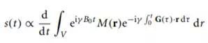
In the presence of this general time-varying gradient, the received signal is
The center frequency γ B0 is always much larger than the bandwidth of the signal. Hence the derivative operation is approximately equivalent to multiplication by −iω0 . The signal is demodulated by the waveform eiγ B0t to obtain the “baseband” signal:

It will be helpful to define the term k(t):
Then we can rewrite the received baseband signal as
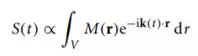
which we can now identify as the spatial Fourier transform of M(r) evaluated at k(t). That is, S(t) scans the spatial frequencies of the function M(r). This can be written explicitly as

where M(k) is the three-dimensional Fourier transform of the object distribution M(r). Thus we can view MRI with linear gradients as a “scan” of k-space or the spatial Fourier transform of the image. After the desired portion of k-space is scanned, the image M(r) is reconstructed using an inverse Fourier transform.