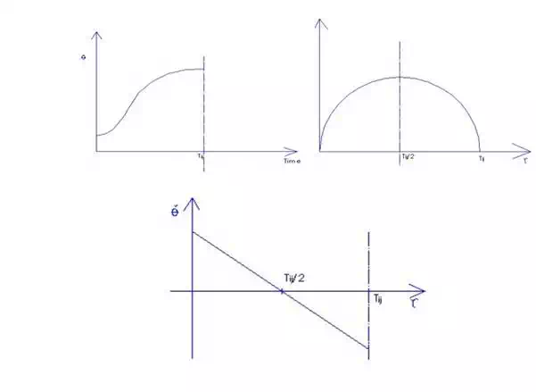
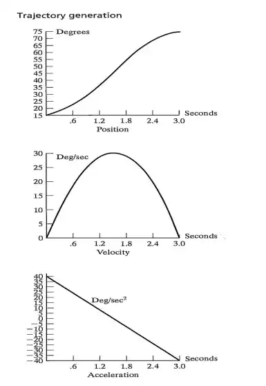
Below Figure shows the position, velocity and acceleration functions for this motion sampled at 40 Hz. Note that the velocity profile for any cubic function is a parabola and that the acceleration profile is linear.
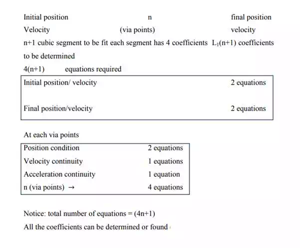
User specify n+2
Final position
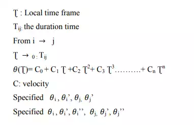
Position velocity User has to give Cartesian data and large data which is kinematically consistent:
Another constraints ![]() user interface must be simple
user interface must be simple
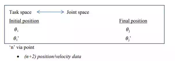
User should specify the following for creating trajectory:
· Initial position
· Final position
· Via points
Notice: Position specifies velocity to be chosen by the system.
Example:
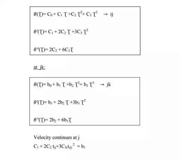
3 points specified i, j, k
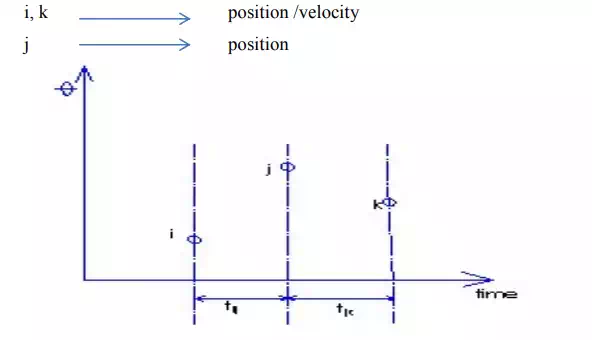
this picture specifies time with respect of speed
Two cubic curves (segment)
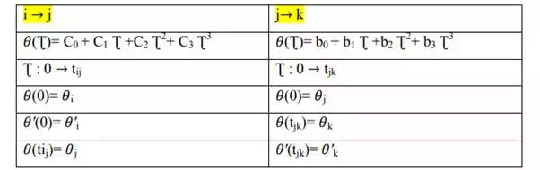
at j:
Continuity of velocity and acceleration