
The root locus is a graphical representation in s-domain and it is symmetrical about the real axis. Because the open loop poles and zeros exist in the s-domain having the values either as real or as complex conjugate pairs. In this chapter, let us discuss how to construct (draw) the root locus.
Rules for Construction of Root Locus
Follow these rules for constructing a root locus.
Rule 1 − Locate the open loop poles and zeros in the ‘s’ plane.
Rule 2 − Find the number of root locus branches.
We know that the root locus branches start at the open loop poles and end at open loop zeros. So, the number of root locus branches N is equal to the number of finite open loop poles P or the number of finite open loop zeros Z, whichever is greater.
Mathematically, we can write the number of root locus branches N as
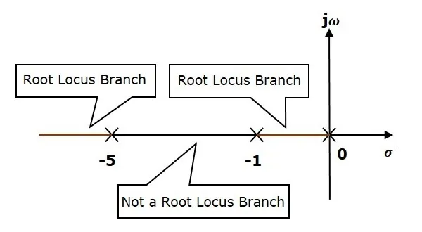
Rule 3 − Identify and draw the real axis root locus branches.
If the angle of the open loop transfer function at a point is an odd multiple of 1800, then that point is on the root locus. If odd number of the open loop poles and zeros exist to the left side of a point on the real axis, then that point is on the root locus branch. Therefore, the branch of points which satisfies this condition is the real axis of the root locus branch.
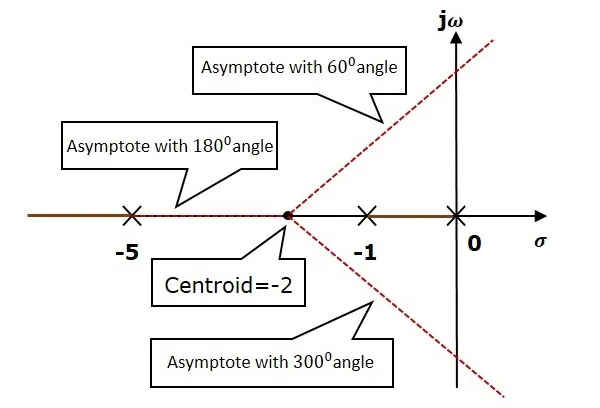
Rule 4 − Find the centroid and the angle of asymptotes.
· If P=Z, then all the root locus branches start at finite open loop poles and end at finite open loop zeros.
· If P>Z, then Z number of root locus branches start at finite open loop poles and end at finite open loop zeros and P−Z number of root locus branches start at finite open loop poles and end at infinite open loop zeros.
· If P<Z , then P number of root locus branches start at finite open loop poles and end at finite open loop zeros and Z−P number of root locus branches start at infinite open loop poles and end at finite open loop zeros.
So, some of the root locus branches approach infinity, when P≠Z. Asymptotes give the direction of these root locus branches. The intersection point of asymptotes on the real axis is known as centroid.
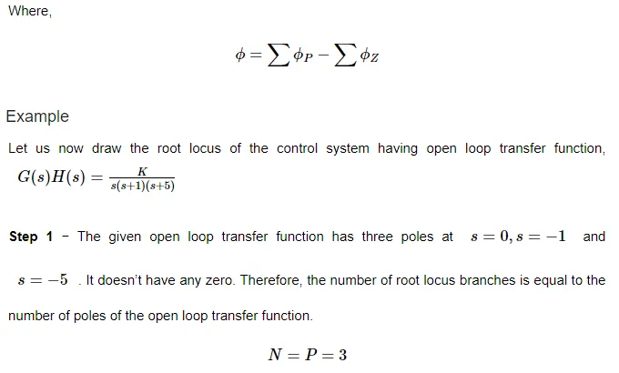
We can calculate the centroid α by using this formula,
In this way, you can draw the root locus diagram of any control system and observe the movement of poles of the closed loop transfer function.
From the root locus diagrams, we can know the range of K values for different types of damping.
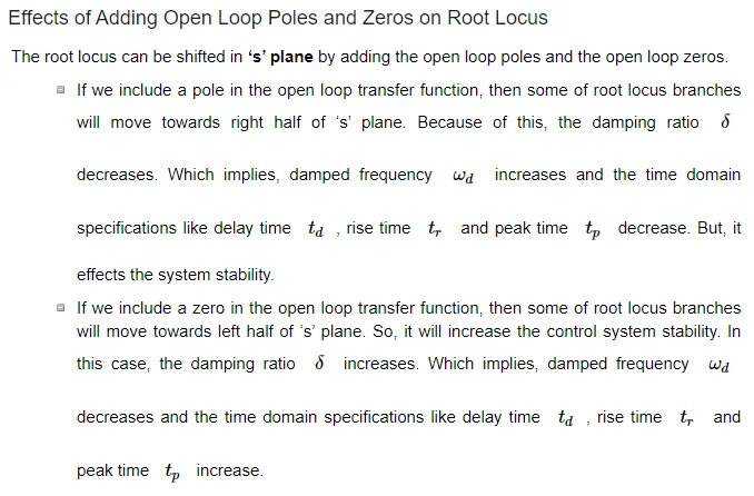
So, based on the requirement, we can include (add) the open loop poles or zeros to the transfer function.