basic / September 5, 2021

Gaussian Elimination Method In 3 × 3 Matrices

Suppose I have a system of equations likeContentsMETHODEXAMPLESOLUTIONSTEP 1STEP 2 How it would be if I want to write it in a matrix form? Well, in the matrix form, it will be Here the coefficient matrix is the variable matrix is and the constant matrix is Now there are several methods to solve a system […]

By senseadmin · September 5, 2021 · 3 min read

Suppose I have a system of equations like

Contents

METHOD

EXAMPLE
SOLUTION

STEP 1
STEP 2

\begin{eqnarray*} a_{11}x_1+a_{12}x_2+a_{13}x_3 &=& b_1\\ a_{21}x_1+a_{22}x_2+a_{23}x_3 &=& b_2\\\ a_{31}x_1+a_{32}x_2+a_{33}x_3 &=& b_3. \end{eqnarray*}

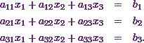
How it would be if I want to write it in a matrix form?

Well, in the matrix form, it will be

\[ \begin{pmatrix} a_{11} & a_{12} & a_{13}\\ a_{21} & a_{22} & a_{23}\\ a_{31} & a_{32} & a_{33} \end{pmatrix}\begin{pmatrix} x_1\\ x_2\\ x_3 \end{pmatrix} = \begin{pmatrix} b_1\\ b_2\\ b_3 \end{pmatrix}. \]

Here the coefficient matrix is

\[ \begin{pmatrix} a_{11} & a_{12} & a_{13}\\ a_{21} & a_{22} & a_{23}\\ a_{31} & a_{32} & a_{33}\end{pmatrix}, \]

the variable matrix is

\[ \begin{pmatrix} x_1\\ x_2\\ x_3 \end{pmatrix} \]

and the constant matrix is

\[ \begin{pmatrix} b_1\\ b_2\\ b_3 \end{pmatrix}.\]

Now there are several methods to solve a system of equations using matrix analysis.

One of these methods is the Gaussian elimination method.

Since here I have three equations with three variables, I will use the Gaussian elimination method in 3 × 3 matrices.

If interested, you can also check out the Gaussian elimination method in 4 × 4 matrices.

METHOD

In this method, first of all, I have to pick up the augmented matrix.

The augmented matrix is the combined matrix of both coefficient and constant matrices.

In this case the augmented matrix $\textbf{A}_b$ is

\[ \textbf{A}_b = \begin{pmatrix} a_{11} & a_{12} & a_{13} & b_1\\ a_{21} & a_{22} & a_{23} & b_2\\ a_{31} & a_{32} & a_{33} & b_3 \end{pmatrix}. \]

Now the job is to get an equivalent upper triangular matrix.

That will be similar to

\[ \begin{pmatrix} a_{11} & a_{12} & a_{13} & b_1\\ 0 & a & b & c\\ 0 & 0 & d & f \end{pmatrix}\text{or}~\begin{pmatrix} a_{21} & a_{22} & a_{23} & b_2\\ 0 & a & b & c\\ 0 & 0 & d & f \end{pmatrix}\]

\[ \text{or}~\begin{pmatrix} a_{31} & a_{32} & a_{33} & b_3\\ 0 & a & b & c\\ 0 & 0 & d & f \end{pmatrix}.\]

After that, I’ll use the backward substitution method to get the values of x_1, x_2, x_3 .

Now I’ll give you an example.

EXAMPLE

According to Stroud and Booth (2011)* “By the method of Gaussian elimination, solve the equations $\textbf{AX} = \textbf{b}$ where

\[ \textbf{A} = \begin{pmatrix} 1 & -2 & -4\\ 2 & 1 & -3\\ 1 & 3 & 2 \end{pmatrix}~\text{and}~\textbf{b} = \begin{pmatrix} -3\\ 4\\ 5 \end{pmatrix}. \]

”

SOLUTION

In this example, the set of equations is $\textbf{AX} = \textbf{b}$ .

Also, I know that the coefficient matrix $\textbf{A}$ is

\[ \textbf{A} = \begin{pmatrix} 1 & -2 & -4\\ 2 & 1 & -3\\ 1 & 3 & 2 \end{pmatrix}. \]

In the same way, I also know that the constant matrix $\textbf{b}$ is

\[ \textbf{b} = \begin{pmatrix} -3\\ 4\\ 5 \end{pmatrix}. \]

Now I have to solve this set of equations. This means I have to get the value of the matrix $\textbf{X}$ .

Let me choose $\textbf{X}$ as

\[ \textbf{X} = \begin{pmatrix} x_1\\ x_2\\ x_3 \end{pmatrix}. \]

As I have mentioned earlier, the first step is to convert the augmented matrix $\textbf{A}_b$ to an upper triangular matrix.

STEP 1

Now the augmented matrix $\textbf{A}_b$ is

\[ \textbf{A}_b = \begin{pmatrix} 1 & -2 & -4&-3\\ 2 & 1 & -3&4\\ 1 & 3 & 2&5 \end{pmatrix}. \]

First of all, I’ll subtract twice row 1 from row 2.

Simultaneously, I’ll also subtract row 1 from row 3.

In mathematical term, I’ll write it like this:

Row 2 – 2(Row 1), Row 3 – Row 1.

Thus the equivalent matrix will be

\[ \textbf{A}_b \thicksim \begin{pmatrix} 1 & -2 & -4&-3\\ 0 & 5 & 5&10\\ 0& 5 & 6&8 \end{pmatrix}. \]

Next, I’ll divide row 2 by 5.

$\cfrac{1}{5}$ Row 2 gives

\[ \textbf{A}_b \thicksim \begin{pmatrix} 1 & -2 & -4&-3\\ 0 & 1 & 1&2\\ 0& 5 & 6&8 \end{pmatrix}. \]

Then I’ll subtract 5 times row 2 from row 3.

Thus Row 3 – 5 (Row 2) gives

\[ \textbf{A}_b \thicksim \begin{pmatrix} 1 & -2 & -4&-3\\ 0 & 1 & 1&2\\ 0& 0 & 1&-2 \end{pmatrix}. \]

This is the upper triangular form of the matrix.

Therefore the system of equations in the matrix form is

\[ \begin{pmatrix} 1 & -2 & -4\\ 0 & 1 & 1\\ 0& 0 & 1 \end{pmatrix}\begin{pmatrix} x_1\\ x_2\\ x_3 \end{pmatrix} = \begin{pmatrix} -3\\ 2\\ -2 \end{pmatrix}. \]

Now my next job is to solve this system.

STEP 2

Here I’ll use the backward substitution to solve these equations.

This means I’ll start from the bottom.

Now the equations are

(1) $\begin{equation*} (1). x_1 + (-2). x_2 + (-4). x_3 = (-3), \end{equation*}$

(2) $\begin{equation*} (1). x_2 + (1). x_3 = 2, \end{equation*}$

(3) $\begin{equation*} (1). x_3 = -2. \end{equation*}$

Therefore from equation (3), I can say that

Next, I’ll substitute x_3 = -2 in equation (2).

Thus it will be

\begin{equation*} (1). x_2 + (1). (-2) = 2. \end{equation*}

Now I’ll simplify it to get the value of x_2.

\begin{eqnarray*} (1). x_2 + (1). (-2) &=& 2\\ x_2 -2 &=& 2\\ x_2 &=& 4. \end{eqnarray*}

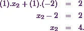
At the end, I’ll substitute x_2 = 4 and x_3 = -2 in equation (1) to get

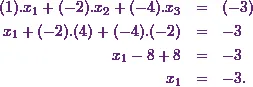
\begin{eqnarray*} (1). x_1 + (-2). x_2 + (-4). x_3 &=& (-3)\\ x_1 + (-2). (4) + (-4). (-2) &=& -3\\ x_1 - 8 +8 &=& -3\\ x_1 &=& -3. \end{eqnarray*}

Hence I can conclude that the variable matrix $\textbf{X}$ is [-3, 4, -2]^T.

This is the solution to this example.